In an earlier post we showed that, for a tax-paying firm, WACC is always a declining function of leverage.  If firm value is an inverse function of WACC, this suggests funding operations with 100% debt.

In fact we observe that firm value is concave in leverage and appears to peak when there is some equity in the capital structure.  We’re forced to conclude that firm value isn’t solely a function of WACC, but instead varies in a more complicated fashion with leverage.  In this post we’ll review one theory that explains this, and which can guide us in divining an “optimal” capital structure.

Financial Distress

Standard WACC theory does not allow for a reduction in operating cash flows as capital structure changes:  as we change leverage in a firm, the only impacts are on division of claims between debt- and shareholders, and on the interest expense tax shield.

However we find that firm value peaks at less than 100% debt.  The only way to achieve this result is to violate one of the Modigliani-Miller assumptions, and model asset flows as depending on leverage.  We will assign two types of costs to financial distress.  Bankruptcy costs cover legal expenses of Chapter 11 filings.  They usually constitute less than 1% of the pre-distress value of a firm, and we ignore them for the balance of this post.

Business disruption costs quantify the reduction in operating asset cash flows as leverage increases.  These costs can rise to over 30% of firm value (Korteweg, The costs of financial distress across industries, 2007).  A common case study is Chrysler during its 1979 distress, when it lost an estimated 5.1% of sales due to perceived distress.  These costs reflect opinions by customers, vendors, and management that the firm may not survive.  These costs begin to occur well before default or bankruptcy, and in fact can help drive an otherwise solvent firm into bankruptcy.

Aside:  Can we model these financial distress costs through increased costs of borrowing — the yield on debt?  Importantly, no:

• Though the riskiness (and cost) of debt may rise with leverage, it can never exceed the riskiness of the unlevered assets.  (In the extreme case, that of 100% leverage, the debt absorbs all firm profits:  the debt has become equity.  In this situation debt risk equals the unlevered asset risk, and debt yield equals the required return on assets.)
• As we add leverage, can we increase asset risk?  Again, no, because throughout the WACC framework what we call asset risk (which is identical to WACC under a 0% tax rate) is the unlevered asset risk.  Asset risk in the WACC framework, by definition, is independent of capital structure.

A Model of Business Disruption Costs

Models of financial distress costs are limited; most published work tries merely to document empirical cases.  Since these costs are driven primarily by psychological factors, they are notoriously difficult to predict.

Hayne Leland (1994) provides a model which allows us to calculate firm value, as a function of leverage, when business disruption costs are present.  The model is slightly revised by Copeland et al., and includes the following assumptions:

1. Firm value follows a geometric Brownian motion diffusion (similar to the behavior of the underlier in the Black-Scholes option pricing model)
2. When firm value falls to the value of debt, business disruption costs (expressed as a percentage of unlevered firm value) result.  As referenced above, these costs can be 30% or more.  Additionally, at this point any interest expense tax shield is no longer enjoyed.
3. Regardless of leverage, the firm’s debt (face value D) always pays the same coupon (risk-free rate).  We express debt risk as a reduction in market value of the debt (B), so that B < D, which produces a cost of debt that rises with leverage.

The model expresses levered firm value as follows:

V_L = V_U + T B – p T B – p a V_B

with the following interpretation:

V_L is the value of the levered firm

V_U is the value of the unlevered firm (all-equity financed, no possibility of business disruption costs occurring)

T is the tax rate

B is the market value of debt

p (between 0 and 1) combines the likelihood and present value impacts of future business disruption.  It is a function of leverage.

a (between 0 and 1) gives the fraction of firm value destroyed by default; it is assumed

V_B is default boundary; often assumed to be the face value of debt

The first two of the four terms give the levered levered firm the same value that the Modigliani-Miller framework provides.  The third term reduces the value of the tax shield for distress; the fourth term reduces the value of the operating assets for distress.

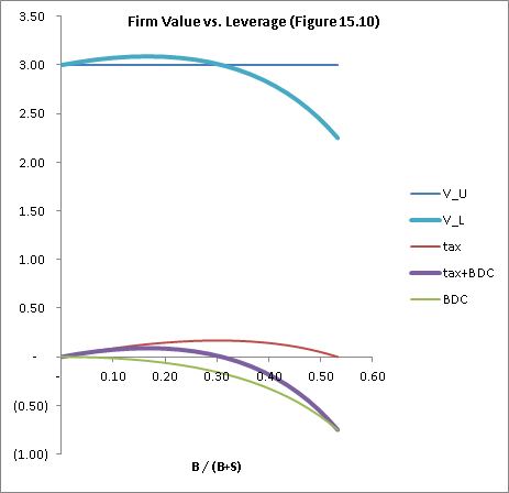
We provide an implementation of the model here:  [download id=”7″].  For a=30% and certain assumptions about the volatility of firm value, we obtain the following chart:

In this example, V_L is maximized at 17% leverage (defined as the ratio of market value of debt to total capitalization).

There are some notable conclusions of the model:

1. Tax shields only exist when the firm generates pretax income; thus the expected value of tax shields peaks at less than 100% leverage.  (In the chart above, they peak at 30% leverage; they are exhausted at 53% leverage.)
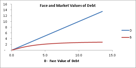
2. The value of debt is less than its nominal (face) value.  The model supports, for example, putting $5 of debt onto a firm with $3 of asset value.  The debt will be valued at something less than the unlevered asset value (though close to it), and equity will have a small positive value reflecting the possibility that V could some day rise above $5.  The following chart shows this relationship:  
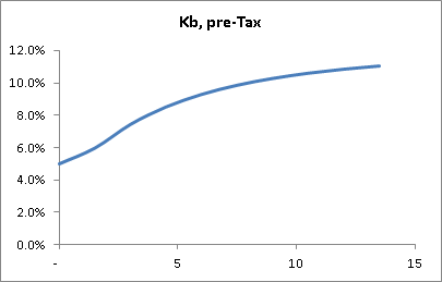
3. The cost of debt rises from the risk-free rate toward the cost of assets (12% in the example) as a function of leverage:  

Recipe

Applying this model to a specific situation requires a few steps:

1. Input parameters:   The blue cells in the spreadsheet indicate input assumptions.   Several of these (face value of debt, tax rate, risk-free rate, levered firm value) can be observed and entered directly.
2. Of the remaining model parameters (V_U, rho, sigma, alpha, debt maturity, default boundary), calculate what you can from analysis.  For example, rho (required return) could be derived from the (unlevered) cost of assets for other firms in the same industry.  V_U could be calculated using a DCF analysis of the asset’s cash flows.
3. Since the model’s output (levered firm value) is directly observable (as the firm’s enterprise value), it’s possible to construct a system of equations with your remaining unknowns, and solve the system simultaneously.
   1. Alternately, you could sensitize to values for the unknown inputs; for example, execute the model for varying values of alpha.